Tutorial 4 — Two-Stage Stochastic Optimisation

The previous tutorials optimise against a single year. But the right investment under 2023 prices may be wrong under 2025 prices. Two-stage stochastic optimisation finds one set of investment decisions (here-and-now) that performs best in expectation across several scenarios, while dispatch adapts per scenario (wait-and-see).

We reuse the brownfield plant from Tutorial 2 — Brownfield & Process Constraints and optimise it across three weather/market scenario years (2022 / 2023 / 2024) at once.

—

1 · The two-stage idea

\[\min_{\text{capacities}}\; \sum_{s} p_s \, \big[\, \text{CAPEX}^{\text{ann}} + \text{OPEX}_s \,\big]\]

Investment variables are shared across scenarios \(s\) (you build one plant); operational variables are scenario-specific (each year is dispatched on its own prices and renewable profiles). Scenarios carry a probability \(p_s\) summing to 1. The objective is the expected annual cost.

—

2 · Run it

cp tutorials/4_stochastic/config.yaml   config/config.yaml
cp tutorials/4_stochastic/n_config.yaml config/n_config.yaml
snakemake --cores 4     # downloads/preprocesses all scenario years first

stochastic:
  stochastic: true
  EVPI: false
  # scenarios 2022/2023/2024 and their weights are set in config.default.yaml

Stochastic needs a pure LP — two required changes

The tutorials/4_stochastic/n_config.yaml already applies these; they are the reason it differs from the Tutorial 2 brownfield n_config:

1. No unit commitment — committable: false everywhere (stochastic cannot use binary variables).

2. No ramp limits — set ramp limit up / ramp limit down to null for electrolysis, methanolisation and biomethanation. PyPSA (≤ 1.2.2) cannot build ramp-limit constraints on a scenario network, and a value such as 1 still builds them — only null disables them. See Stochastic Optimisation → Limitations.

The output folder uses the STC token instead of DET. Temporal resolution is set to 3h to keep solve time manageable.

—

3 · Interpret the results

The three scenarios span very different market conditions (2022 = energy-crisis year; 2023/2024 = post-crisis normalization), with weights 10 % / 40 % / 50 %:

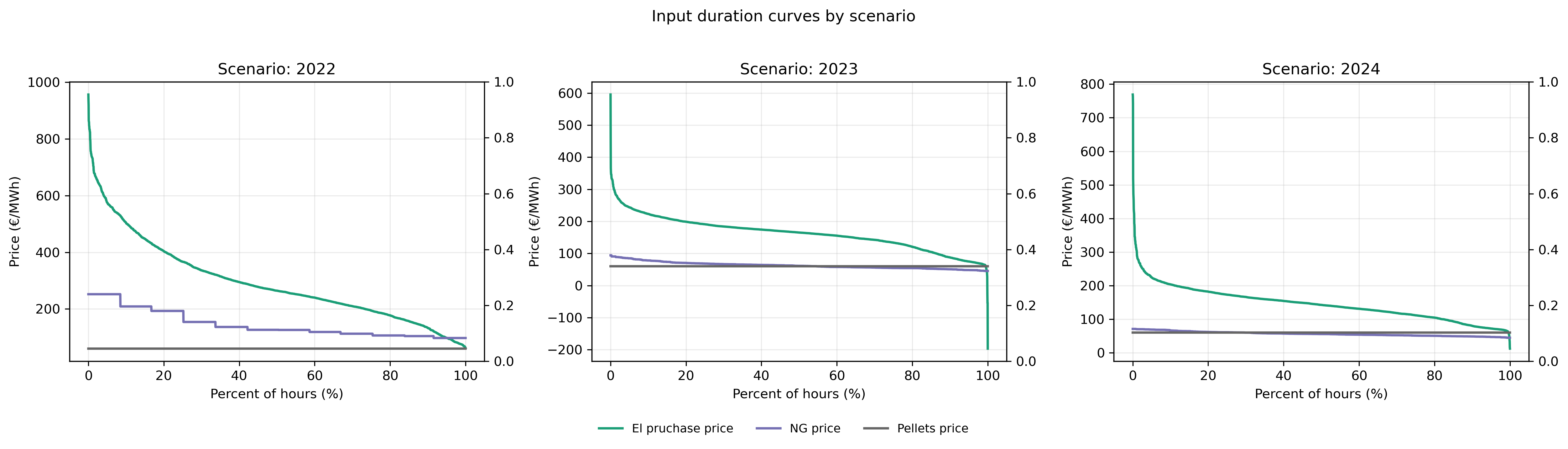
Input duration curves for all three scenarios. 2022 was the European energy-crisis year — elevated NG and biomethane prices made this by far the most profitable scenario (€30.0 M/y net). 2023 and 2024 show post-crisis normalization (€5.4 M/y and €3.5 M/y). The 90 % combined weight on 2023/2024 governs the final design.

The optimizer finds one investment that is robust across all three years:

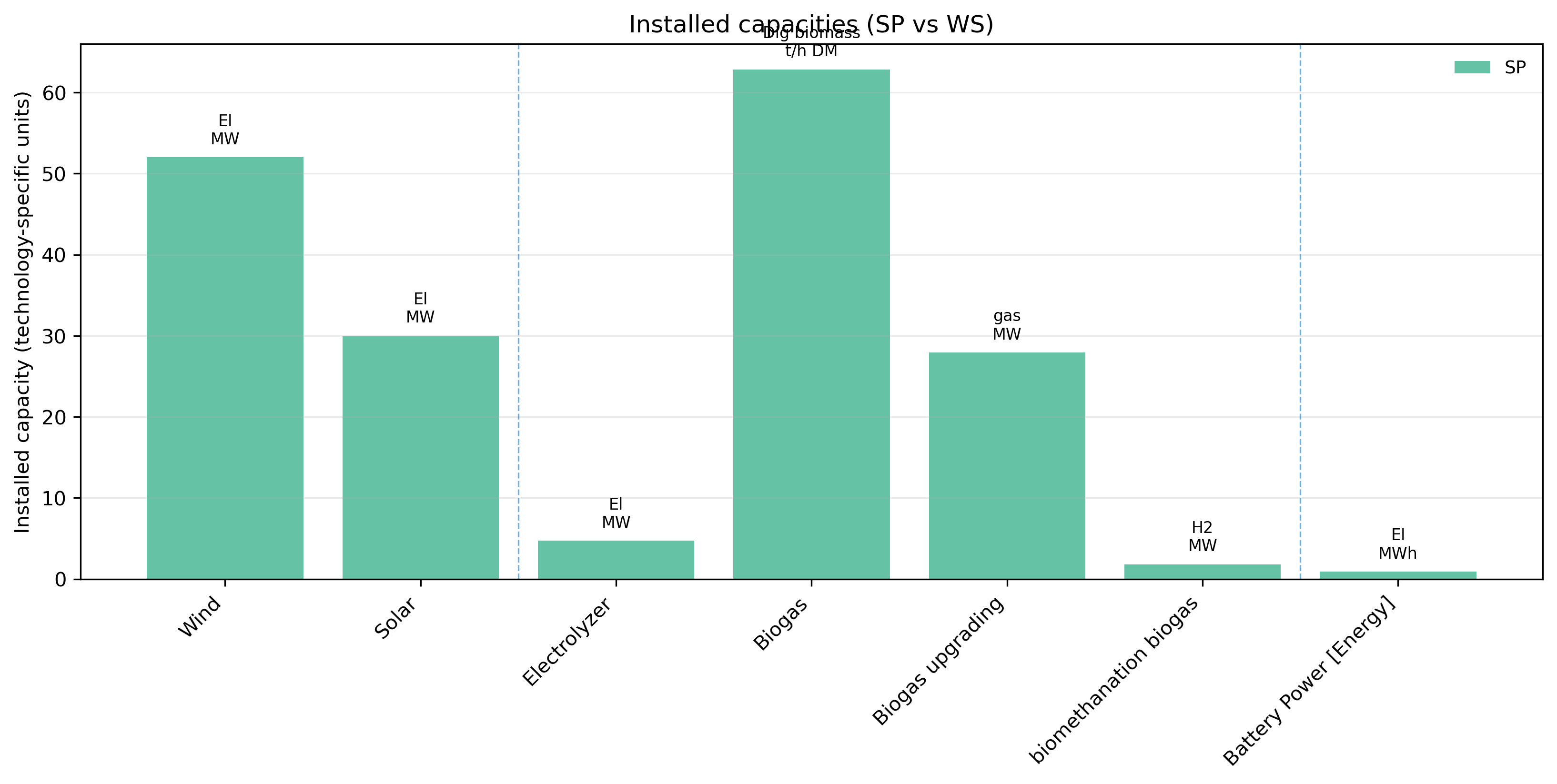
Stochastic-programme (SP) optimal investments: electrolyser 4.7 MW, biogas upgrading 27.9 MW, biomethanation 1.8 MW, battery 0.9 MWh. Existing brownfield assets (52 MW wind, 30 MW solar, 62.85 t/h DM biogas digester) carry over from Tutorial 2.

The expected cost breakdown reveals which revenue streams justify the design:

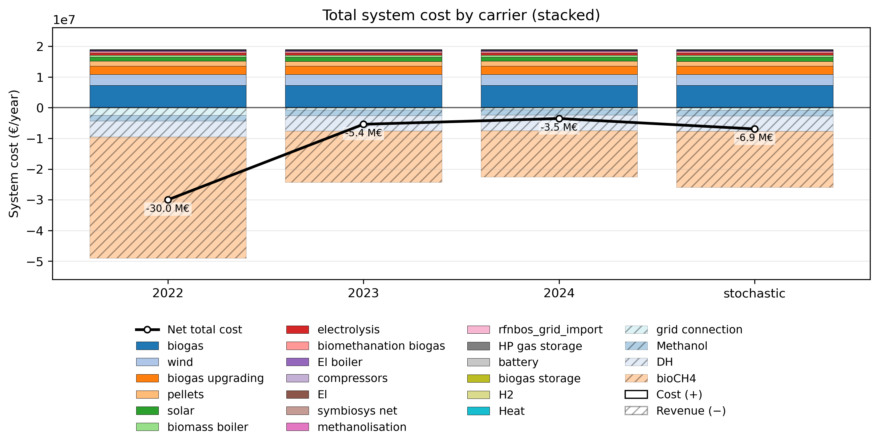
Expected total system cost (probability-weighted) by carrier/agent. Biomethane export (bioCH4) dominates revenues at ≈ €18.1 M/y, followed by district heating (€5.1 M/y) and methanol (€1.8 M/y). Fixed CAPEX (€16.0 M/y, identical across scenarios) is largely the brownfield wind, solar and biogas-digester assets. Expected net profit: €6.9 M/y.

Shadow prices show the internal marginal value of each carrier:

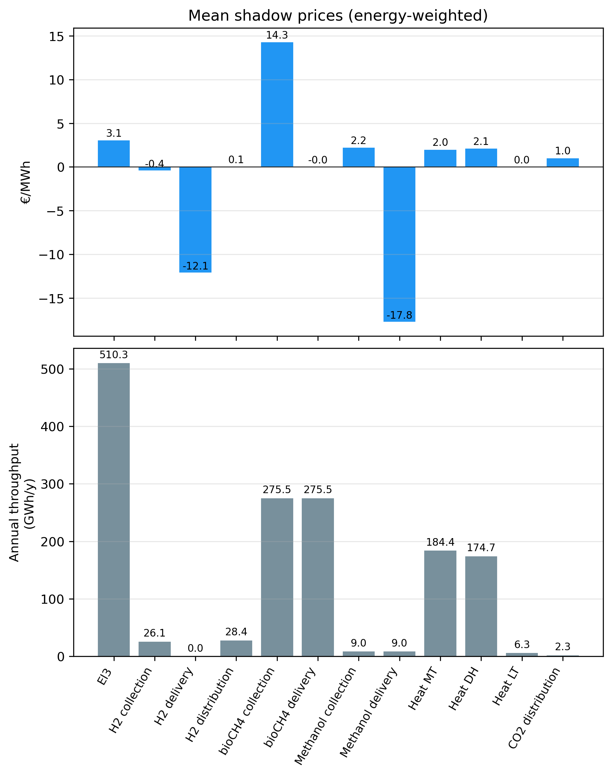
Energy-weighted mean shadow prices and annual throughput. Biomethane collection (€14.3/MWh) is the marginal cost of routing additional biogas to upgrading. The negative H₂ delivery price (−€12.1/MWh) reflects hydrogen’s role as a consumed intermediate in biomethanation rather than a delivered product.

The same fixed-capacity plant dispatches differently in each scenario:

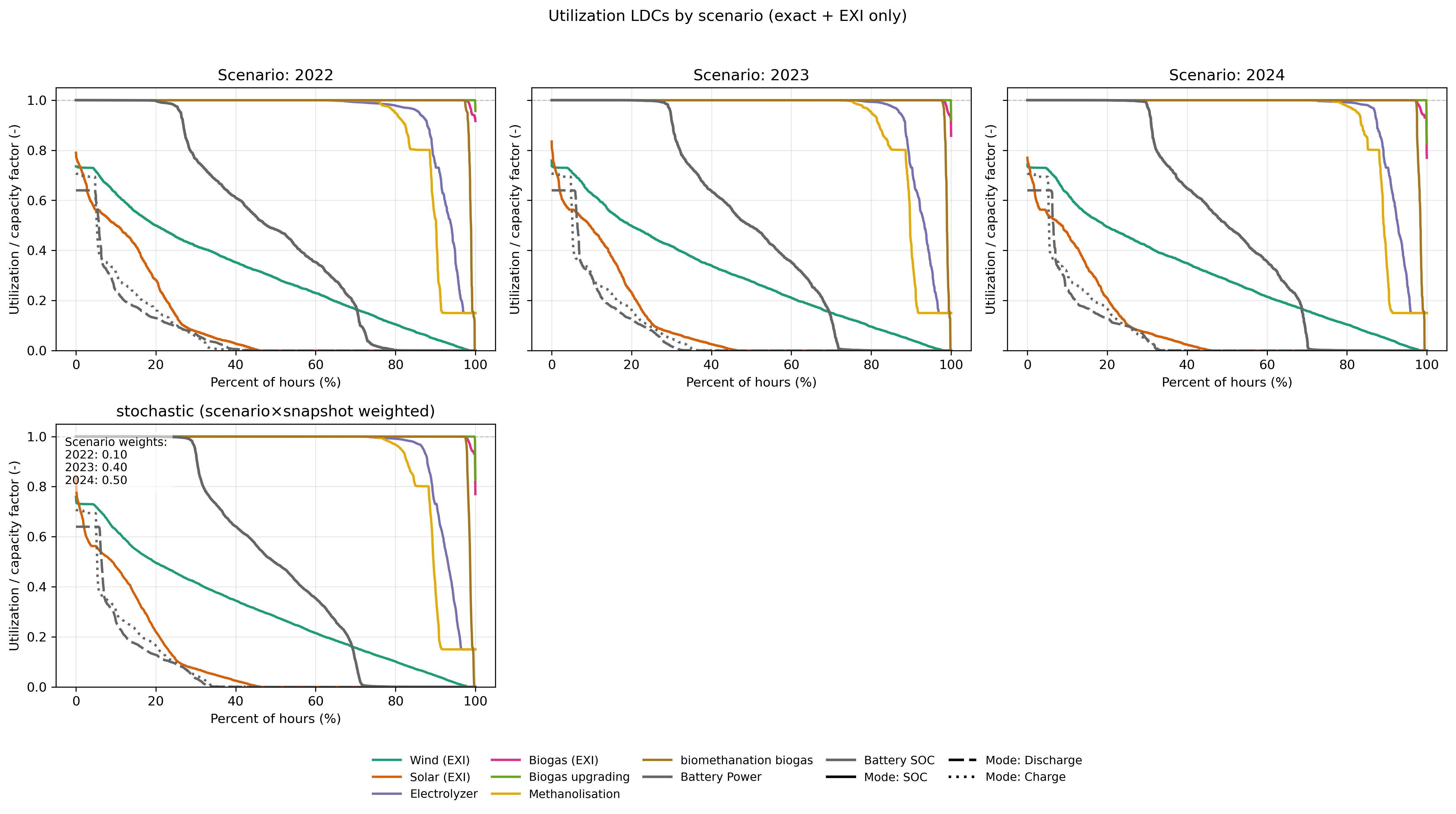
Per-scenario utilization duration curves. Biogas upgrading runs near full capacity year-round in all three scenarios. The small electrolyser (4.7 MW) operates more intensively in 2022 (cheap/negative electricity hours) and more selectively in 2023–2024.

Key results

• Expected net profit: €6.9 M/y (0.10 × €30.0 M + 0.40 × €5.4 M + 0.50 × €3.5 M). The 2022 energy-crisis scenario is far more profitable but carries only 10 % weight; the design is governed by 2023–2024 conditions.

• The stochastic design is a hedge: biogas upgrading (27.9 MW) is built fully because it earns robust revenue in all three years. The electricity-sensitive electrolyser (4.7 MW) is small — sized to exploit cheap-electricity hours without over-betting on any single price environment. Biomethanation is minimal (1.8 MW) for the same reason.

• The same capacity runs very differently across years: the electrolyser is used more aggressively in 2022, more selectively in 2023–2024. This wait-and-see dispatch flexibility is what makes the stochastic design viable.

• Here EVPI: false. Set EVPI: true to also solve each year with perfect foresight and quantify the Expected Value of Perfect Information — the annual value of knowing next year’s market in advance.

—

What you learned

• The here-and-now vs wait-and-see two-stage structure and expected-cost objective.

• How to enable stochastic mode and the pure-LP requirements (no committable, null ramp limits).

• Reading a stochastic design as a robust hedge across scenarios, and interpreting scenario-level profitability spreads.

This is the final tutorial in the core sequence. For exploring near-optimal alternatives to a single design, see the near-optimal (MGA) guide.

See also

Stochastic Optimisation · Outputs & Results Reference · stochastic · Tutorial 2 — Brownfield & Process Constraints