Tutorial 1 — Greenfield: Demand vs Price#
Note
Tutorial format. Each tutorial follows the same loop: (1) read the
concept → (2) copy a ready-made config into config/ → (3) run and
interpret the results. Config files live in tutorials/<name>/ and are
copied over the (gitignored) config/config.yaml and
config/n_config.yaml user overrides.
This first tutorial builds the plant from scratch (greenfield: every capacity is an investment decision, nothing pre-exists) and contrasts the two ways GreenBubble can be driven:
1.1 demand-driven — you fix annual production of the three products (H₂ to the grid, biomethane, methanol) and minimise total system cost.
1.2 price-driven — you fix sale prices and let the model decide how much of each product to make to maximise profit.
In both cases every investment must pay back within 10 years
(amortization_period: 10) and only biological methanation
(biomethanation of biogas and of CO₂) is available — the catalytic (Sabatier)
routes are switched off — so we can watch the competition between
biomethanation and biogas upgrading for supplying the biomethane demand.
—
1 · The economic basis#
GreenBubble minimises (demand mode) or maximises the negative of (price mode) the annualised total system cost
Each technology’s investment is turned into a yearly charge with an annuity:
with discount rate \(r\) (discount_rate: 0.07) and lifetime \(n\).
By default \(n\) is each technology’s technical lifetime; here we set
amortization_period: 10 so every technology is amortised over 10 years.
Why this matters
A shorter amortisation period raises the annual capital charge, so the model only builds a technology if it earns its (steeper) payback within 10 years. This is the single most important economic lever in the tutorial — see Economic Assumptions for the full treatment.
—
2 · Run it#
1.1 — demand-driven
cp tutorials/1_greenfield_demand/config.yaml   config/config.yaml
cp tutorials/1_greenfield_demand/n_config.yaml config/n_config.yaml
snakemake --cores 4
Key settings (config.yaml,
n_config.yaml):
targets:
  driver: demand
  demand_H2:   200000     # MWh/y to the grid
  demand_CH4:  350000     # MWh/y biomethane
  demand_meoh:   9000     # MWh/y methanol
  CH4_demand_mode:  flat       # constant demand
  MeOH_demand_mode: bins_flat  # stepwise (bins) demand
amortization_period: 10
The two demand shapes shown — flat (constant every hour) and
bins_flat (a few constant steps) — are the two simplest of the four modes;
see Setting Product Demands for profile and bins_profile.
1.2 — price-driven
cp tutorials/1_greenfield_price/config.yaml   config/config.yaml
cp tutorials/1_greenfield_price/n_config.yaml config/n_config.yaml
snakemake --cores 4
targets:
  driver: price
  price_H2:      120        # EUR/MWh
  price_bioCH4:  200        # EUR/MWh
  price_meoh:    200        # EUR/MWh
  demand_H2:   200000       # now an UPPER BOUND on production
In demand mode the demand_* values are equality constraints (you must
deliver exactly that much). In price mode they become upper bounds: the
model produces a product only while its sale price exceeds its marginal +
annualised capital cost, so price mode reads out the break-even of each route.
Note
Both runs use clustering.temporal.resolution: 3h and the default HiGHS
solver so they finish in a few minutes on a laptop. Outputs land in
outputs/single_analysis/{run_name}/ (e.g. tut1_demand/). File names
inside encode the full configuration (see Wildcards). The full
configuration is also saved to networks/config_run.yaml inside that
folder.
—
3 · Interpret the results (demand case)#
This is the most detailed walkthrough in the series — later tutorials only revisit what changes. For the full map of the output folder and every file see Outputs & Results Reference. We read six figures in order; the numbers quoted are from the 3 h reference run.
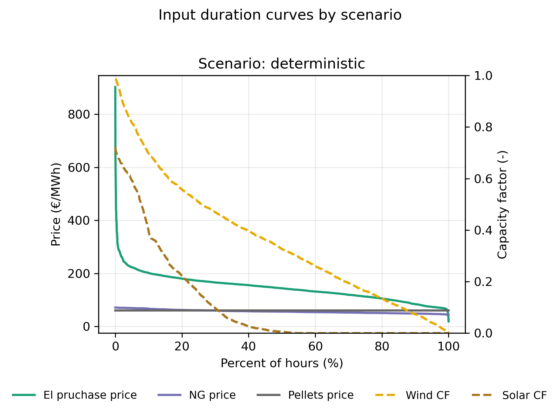
(a) Inputs — the drivers (Inputs — the exogenous drivers). Load-duration curves of electricity price, gas price and wind/solar capacity factors set the economics: how often electricity is cheap decides how attractive electrolysis is.
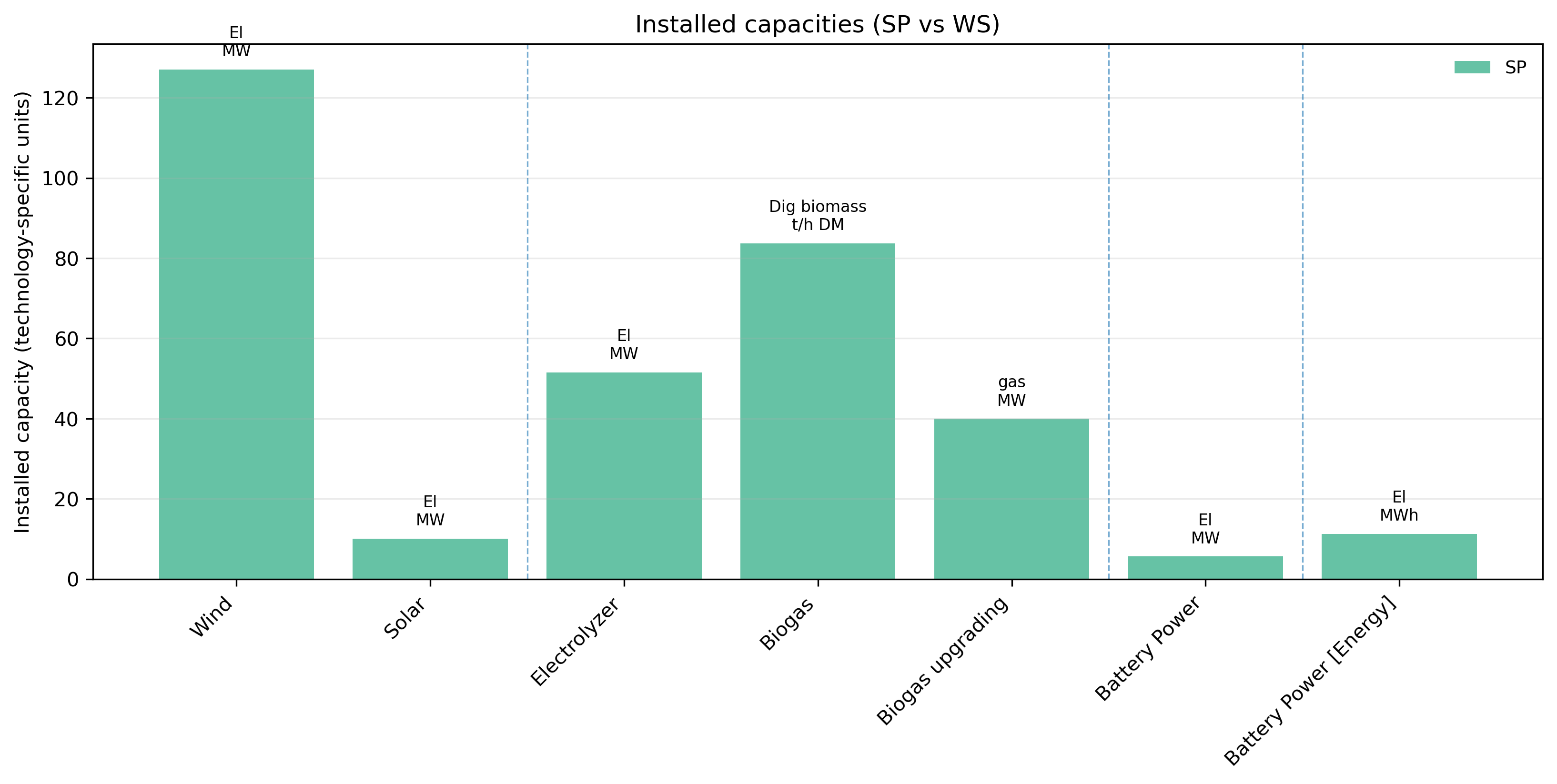
(b) Capacities — what gets built (Capacities — what gets built; data in
optimal_capacities.csv). The model builds 127 MW onshore wind (CF 0.32),
10 MW solar (CF 0.11), a 51.5 MW electrolyser (CF 0.69) and meets the
350 GWh/y biomethane demand with 40 MW of biogas upgrading running near
flat-out. Biomethanation is not built — at default costs biogas upgrading is
the cheaper biomethane route within a 10-year payback window.
Biomethanation vs biogas upgrading — the key result
Both routes deliver pipeline-grade biomethane: upgrading strips CO₂ out of biogas (cheap, but carbon is vented → lower CH₄ yield); biomethanation reacts that CO₂ with green H₂ into extra CH₄ (higher yield, but needs an electrolyser and electricity).
At default costs with a 10-year payback, biogas upgrading wins outright: biomethanation is not built at all (0 MW). The electrolyser that is built (52 MW) serves the H₂-to-grid and methanol demands, not methanation. So the “competition” resolves decisively in favour of upgrading here — the extra CH₄ from biomethanation does not pay back the H₂ + reactor cost within 10 years.
To make biomethanation competitive: increase price_bioCH4, lower
amortization_period further, or add CO₂ utilisation incentives.
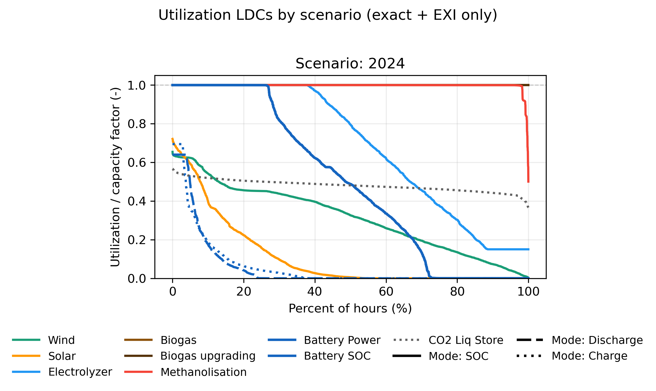
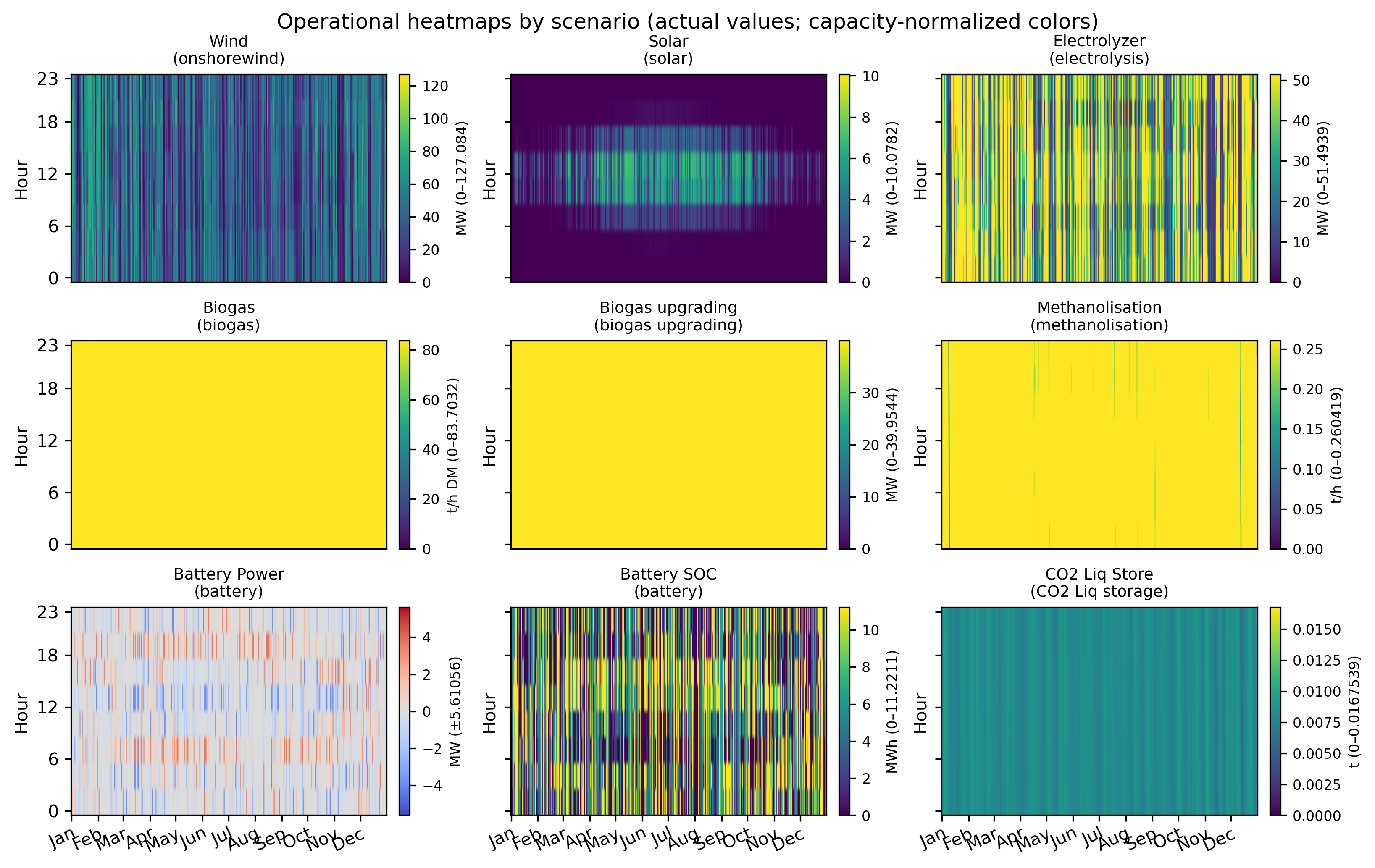
(c) Operation — how it runs (Operation — how it runs). Capacity factors show how hard each asset works; the heat maps show when. The electrolyser runs at CF 0.69, following cheap-power hours; upgrading runs near-constantly.
(d) Internal-market shadow prices (Internal-market shadow prices; data in
shadow_prices_mean.csv). In demand mode these are the marginal cost of
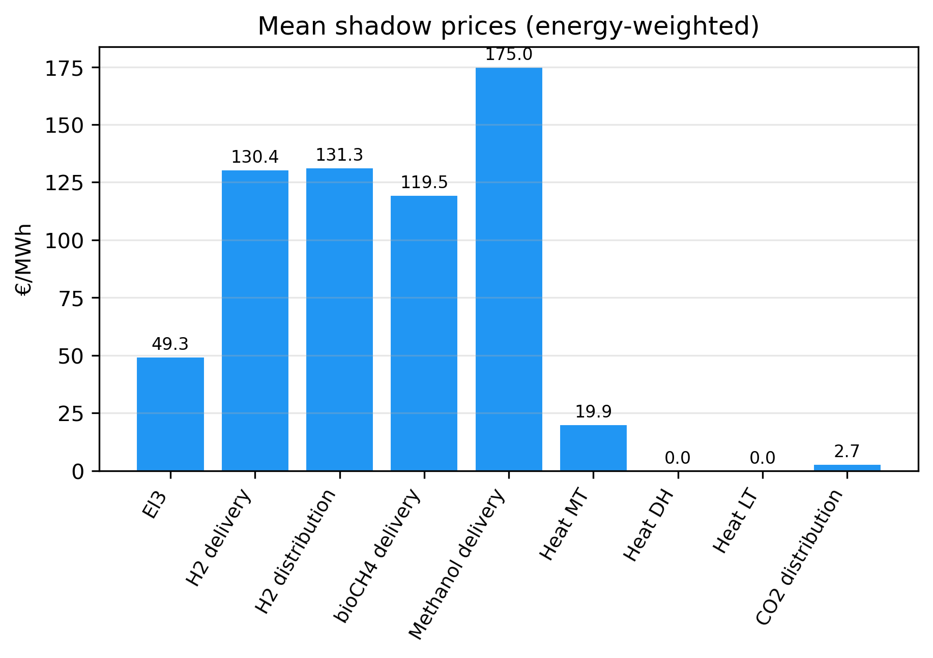
meeting each product’s demand: H₂ ≈ 130 €/MWh, biomethane ≈ 119 €/MWh,
methanol ≈ 175 €/MWh; internal CO₂ ≈ 2.7 €/MWh and medium-temperature heat
≈ 20 €/MWh. The time-resolved srmc_by_technology.png (SRMC & merit order)
shows which units are in merit hour by hour.
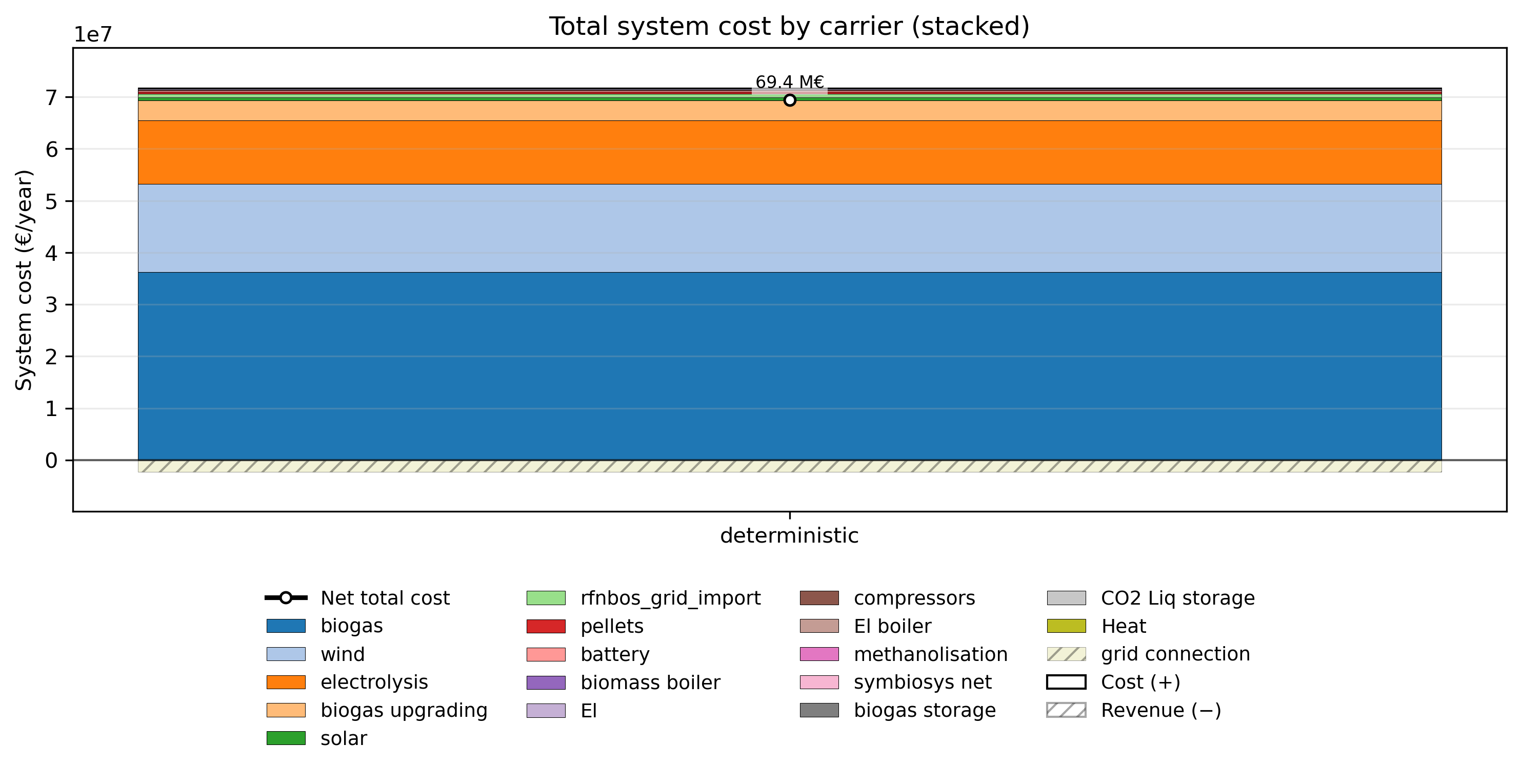
(e) Total system cost (System cost & levelised cost; data in TSC_by_carrier.csv).
Net total ≈ €69.5 M/y, dominated by the biogas plant CAPEX, then wind,
electrolysis and upgrading, with a small grid-export revenue. In demand
mode each product’s LCOP equals its delivery shadow price (bioCH₄ 119, H₂ 130,
MeOH 175 €/MWh) — the zero-profit signature of a cost-minimising solve.
(f) The data behind it all. Every number above aggregates
csv/full_component_table.csv (The master data table) — one row per
component with capacity, capacity factor, costs, production and revenue.
—
4 · The price case#
Re-run with the price-driven config (Section 2): prices price_H2 = 120,
price_bioCH4 = 200, price_meoh = 200 €/MWh. Now production is optional
and driven by profitability — the model maximises profit (net ≈ €28.3 M/y).
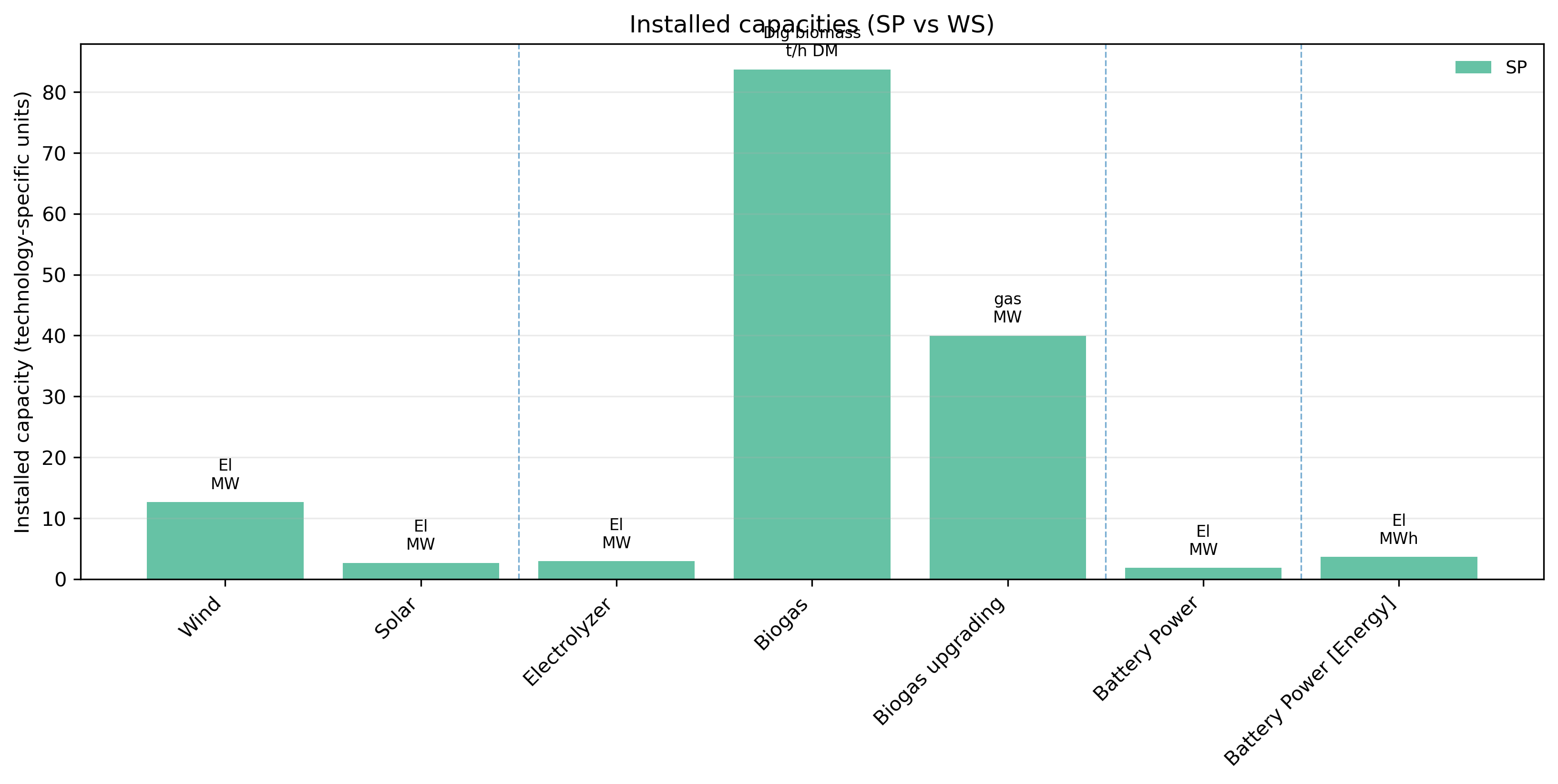
Price-case results
Compare each product’s price against its break-even LCOP from the demand case:
Biomethane (price 200 ≫ LCOP 119) — the big winner: produced up to its cap (350 GWh/y) entirely via biogas upgrading (40 MW, flat). Even at this high price biomethanation is not built — upgrading remains the cheaper route, so the profit-maximiser never needs it.
Methanol (price 200 > LCOP 175) — produced at its full cap (9 GWh/y); a small electrolyser (2.9 MW), wind (12.6 MW) and solar (2.6 MW) are built essentially to feed methanol synthesis.
H₂ to grid (price 120 < LCOP 130) — not profitable at the greenfield cost, so very little is sold: the electrolyser is sized for methanol’s H₂ need only. This is the clearest “price reveals break-even” signal — raise
price_H2above ~130 €/MWh and H₂-to-grid immediately becomes attractive.
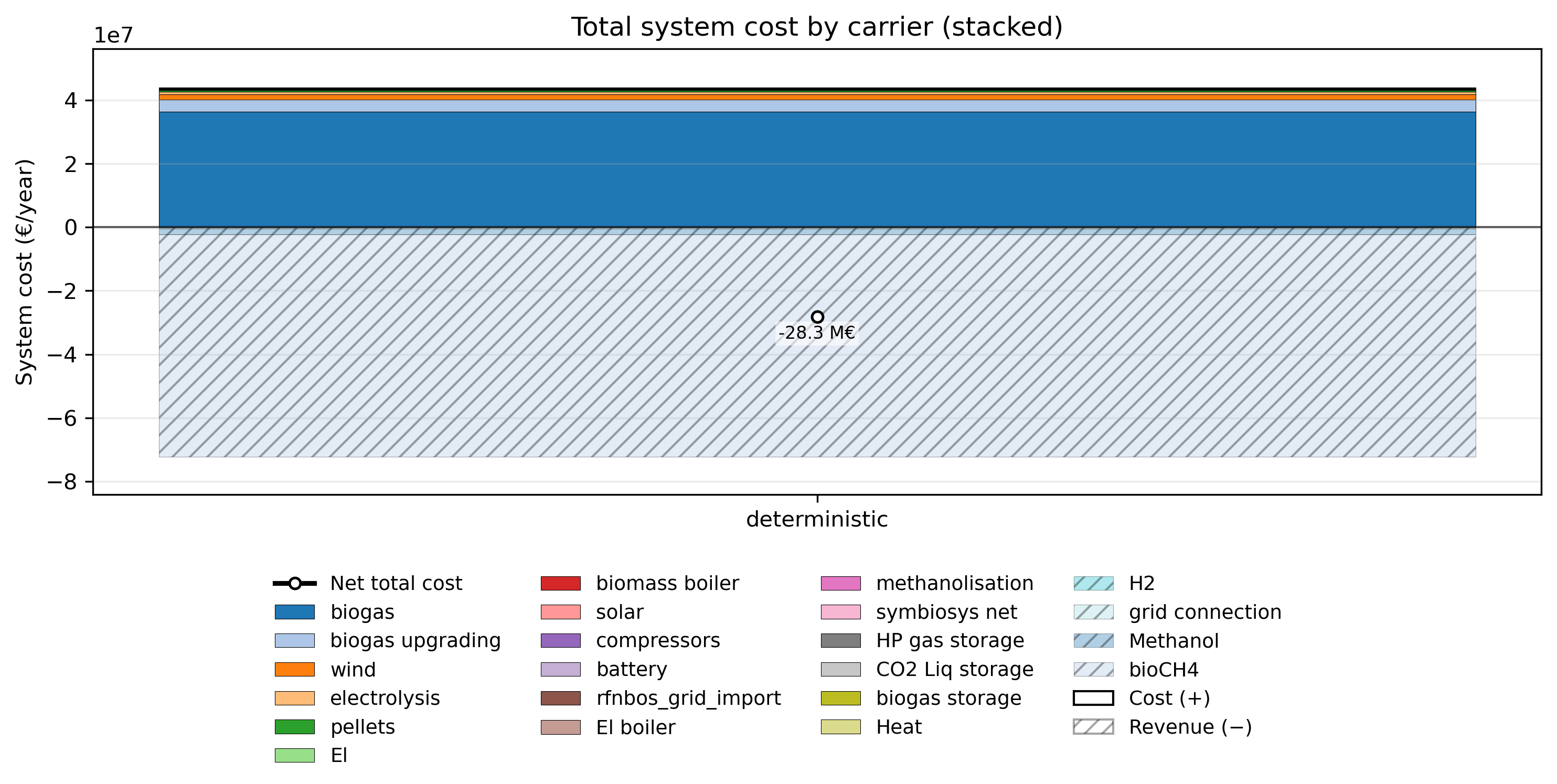
The cost-by-carrier plot now shows revenue bars (products sold) against technology costs; the net is a profit rather than a pure cost.
—
What you learned#
The annuity /
amortization_periodmechanism and why payback length drives what gets built.The difference between demand (fixed production, minimise cost) and price (fixed prices, maximise profit) optimisation.
The biomethanation vs biogas-upgrading trade-off for biomethane supply.
Next: Tutorial 2 — Brownfield & Process Constraints adds existing assets (brownfield) with residual investment costs, and process constraints (committable, ramping, min-load).
See also
Outputs & Results Reference (every result file) · Economic Analysis of Results (theory) · Economic Assumptions · Setting Product Demands · targets · Economics