Tutorial 2 — Brownfield & Process Constraints

Building on Tutorial 1 — Greenfield: Demand vs Price, this tutorial adds existing assets (brownfield) and introduces the process constraints that shape realistic dispatch: committable operation, ramping, and minimum load.

We stay price-driven, drop hydrogen-to-grid (demand_H2: 0), fix a few plant sizes as pre-existing, and enable district heating as a heat off-take.

—

1 · Greenfield vs brownfield

A technology’s investment mode is set by three n_config keys:

initial capacity	expansion	rif	meaning
0	true	0	Greenfield — built from scratch (Tutorial 1)
>0	false	0	Brownfield, sunk — fixed size, no capital charge
>0	false	>0	Brownfield, residual — fixed size, partial capital charge
>0	true	any	Mixed — existing block + expandable new capacity

rif = remaining_investment_fraction: the share of the original investment still being paid off. The annual charge is

\[\text{rif} \times \text{investment}(\text{construction\_year}) \times \text{annuity}(r, \text{amortization\_period}).\]

Because rif is set per technology, each existing asset carries its own residual cost independently.

—

2 · Run it

cp tutorials/2_brownfield/config.yaml   config/config.yaml
cp tutorials/2_brownfield/n_config.yaml config/n_config.yaml
snakemake --cores 4

Existing assets (n_config.yaml):

biogas:   {initial capacity: 30, expansion: false, construction_year: 2020, remaining_investment_fraction: 0.3}
onwind:   {initial capacity: 52, expansion: false, construction_year: 2020, remaining_investment_fraction: 0.5}
solar:    {initial capacity: 30, expansion: false, construction_year: 2020, remaining_investment_fraction: 0.5}
options:
  DH: {enable: true, price: 30}   # district heating off-take at 30 €/MWh

The biogas plant (30 MW CH₄), wind (52 MW) and solar (30 MW) are now fixed; the optimiser sizes only the remaining expandable technologies (electrolyser, biomethanation, storage, …) around them. Each existing asset carries a different residual fraction: the biogas plant recovers 30 % of its original investment, wind and solar 50 %.

—

3 · Process constraints

Three constraints make dispatch physically realistic. They are configured per technology in n_config:

• Committable (committable: true) — binary on/off unit commitment. Only valid for fixed-size components (expansion: false) or rolling horizon, because it turns the problem into a MILP. Leave false for expandable units.

• Ramp limits (ramp limit up / ramp limit down) — max fractional change in output per hour (e.g. 0.9 = 90 %/h for the electrolyser).

• Minimum load (min load) — fraction of capacity that must run when the unit is on (e.g. 0.15 for the electrolyser); below it the unit shuts off.

The common result figures (capacities, operation, shadow prices, system cost) are described once in Outputs & Results Reference and read as in Tutorial 1 — Greenfield: Demand vs Price; below we focus only on what brownfield changes.

—

4 · Interpret the results

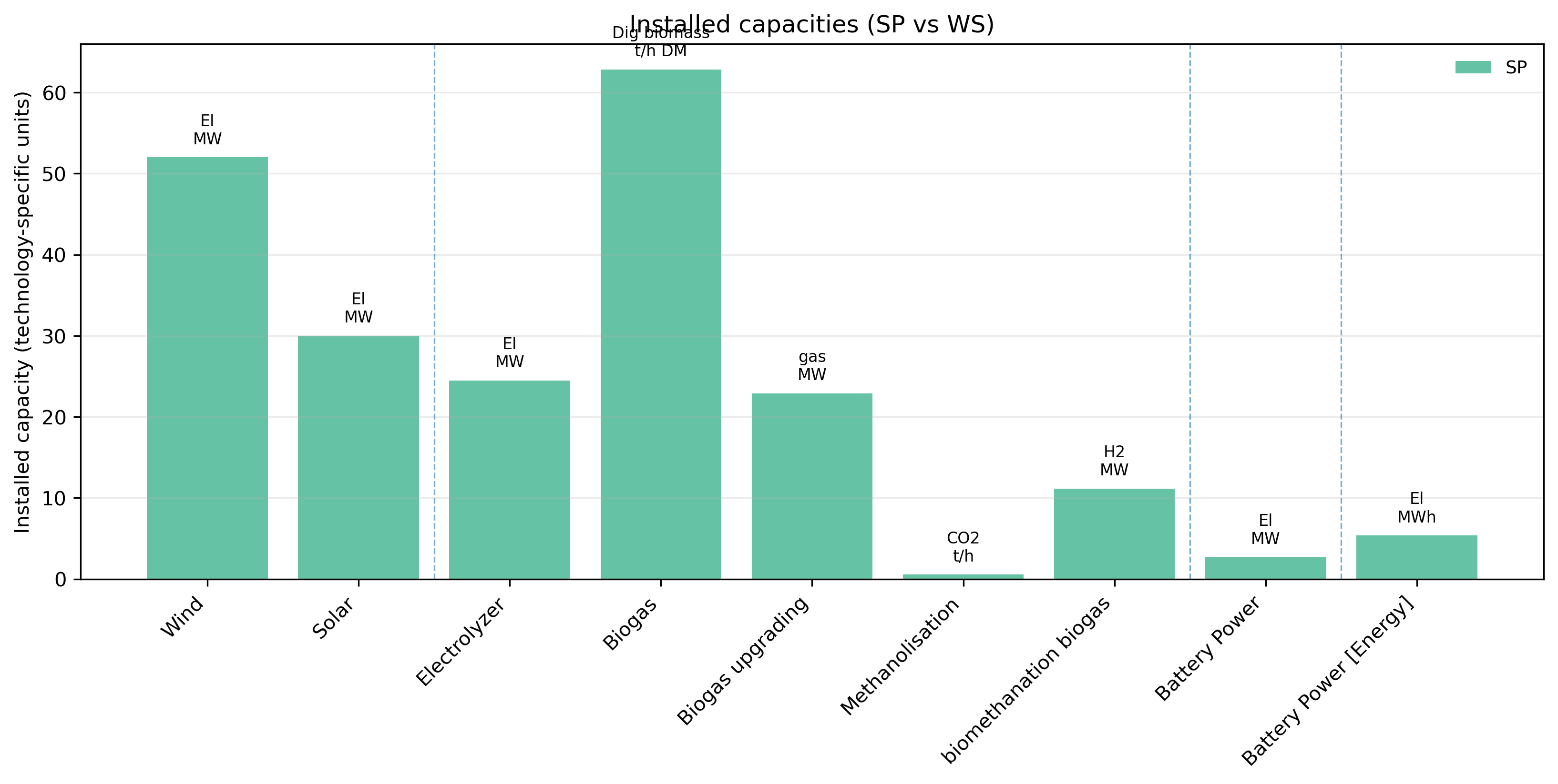
Optimal capacities. The EXI_ assets (biogas 62.85 t/h DM ≈ 30 MW CH₄, wind 52 MW, solar 30 MW) are fixed; everything else is sized around them.

The key change — biomethanation now competes

• Both biomethane routes are built: biogas upgrading 22.9 MW and biomethanation 11.1 MW (vs Tutorial 1, where biomethanation never built). The reason is the fixed, cheap existing renewables: 52 MW wind + 30 MW solar power a 24.5 MW new electrolyser whose H₂ makes extra biomethanation CH₄ worthwhile at price_bioCH4 = 200 €/MWh. The brownfield context is exactly where the upgrading-vs-biomethanation competition turns into a mix.

• District heating adds value to waste heat: the DH bus shadow price clears at ≈ 25 €/MWh and biomethanation/heat-exchanger links export heat to it.

• Net profit ≈ €48.7 M/y — the existing assets are largely sunk, so only their residual CAPEX is charged rather than a full greenfield investment.

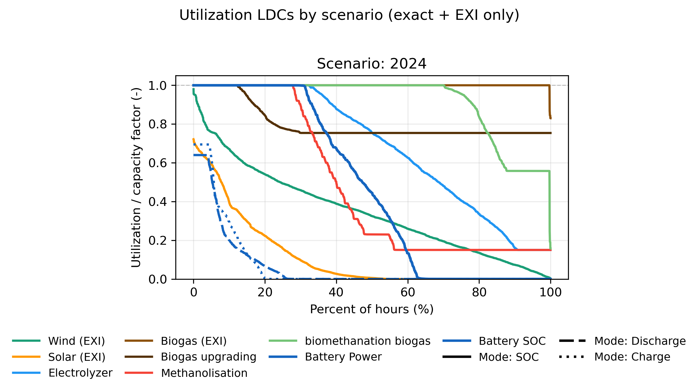
• Electrolyser CF ≈ 0.68, biomethanation CF ≈ 0.92 (running near-constantly wherever H₂ is available), upgrading CF ≈ 0.80.

The process constraints shape how units run: the electrolyser ramps with cheap renewable hours (visible in the operation LDCs below), while upgrading acts as baseload because CO₂ supply is continuous.

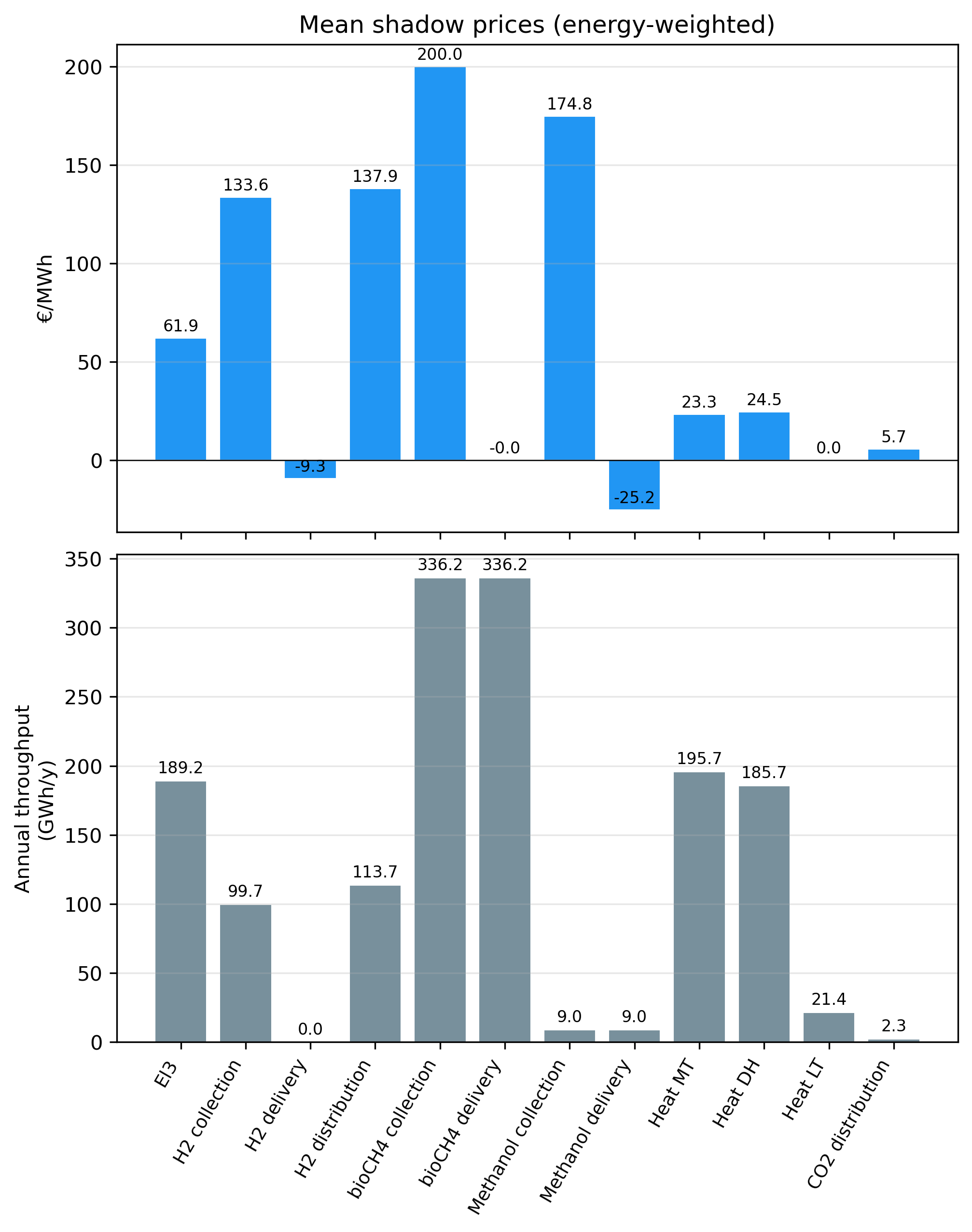
Energy-weighted mean shadow prices at internal carrier buses. Biomethane collection sits at ≈ 200 €/MWh (at its price target), H₂ collection ≈ 134 €/MWh, and heat buses at 23–25 €/MWh.

—

What you learned

• Greenfield vs brownfield vs mixed, and independent residual cost per asset.

• The committable / ramping / min-load process constraints and when each applies.

• Adding a heat off-take (district heating) as a revenue stream.

• Why brownfield context changes the biomethanation break-even.

Next: Tutorial 3 — Rolling Horizon Dispatch re-dispatches this fixed plant hour-by-hour over the full year using rolling horizon, and Tutorial 2b — Heat Network Integration extends the brownfield plant with a larger electrolysis and heat-network integration.

See also

Outputs & Results Reference · Economics · Economic Assumptions · Tutorial 1 — Greenfield: Demand vs Price