Tutorial 3 — Rolling Horizon Dispatch#
Capacity expansion decides what to build; rolling horizon decides how to operate a fixed plant through the year, one sliding window at a time — closer to how a plant is actually run, and without perfect foresight over all 8760 hours.
This tutorial takes the solved brownfield network from Tutorial 2 — Brownfield & Process Constraints and re-solves only its dispatch.
—
1 · How rolling horizon works#
The full year is solved in overlapping windows (here 168 h windows with a
72 h overlap). Each window is optimised with the end-of-previous-window state
as its start; the overlap is discarded to avoid end-of-horizon artefacts.
Capacity expansion is bypassed entirely — capacities are read from the
network_path network and held fixed.
Important
Rolling horizon is dispatch-only and runs at full hourly resolution
(temporal clustering is ignored). It needs a previously solved, fixed-capacity
*_OPT.nc — so run Tutorial 2 first.
—
2 · Run it#
# 1) ensure Tutorial 2 has produced its *_OPT.nc
# 2) point network_path at it (already pre-filled; edit if your path differs)
cp tutorials/3_rolling_horizon/config.yaml   config/config.yaml
cp tutorials/3_rolling_horizon/n_config.yaml config/n_config.yaml
snakemake --cores 4
rolling_horizon:
  enabled:      true
  horizon:      168       # window length (h)
  overlap:       72       # overlap (h)
  rh_year:      2024
  network_path: 'outputs/single_analysis/tut2_brownfield_heat/networks/B_H_RE_H2_METH_SN_ST_CO2_100_tD_H2_580_MeOH_0_CH4_262_2024_El_0.1_DET_3h_tut2_brownfield_heat_OPT.nc'
Committable units are supported in rolling horizon
Unlike stochastic mode, rolling horizon can use unit commitment: each
window is solved as its own (small) MILP, so committable: true on a
fixed-capacity asset is valid here (the min load / committable note in
n_config.default.yaml reads “only for initial capacity or RH”). This
tutorial leaves committable at its default false; you can switch it on for
a fixed (expansion: false) asset to see on/off cycling in the dispatch.
The output network name gets an _RH suffix, and plots land in
outputs/single_analysis/<run_name>/plots_rh/.
—
3 · Interpret the results#
The RH plot suite (in plots_rh/) adds two PF-vs-RH comparison figures.
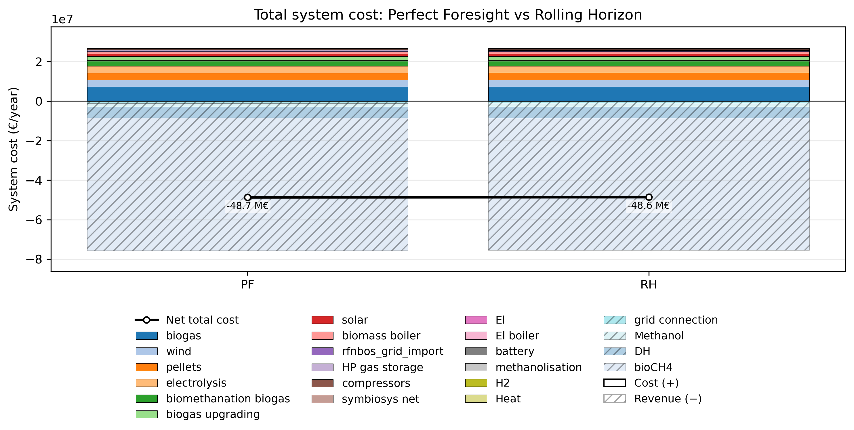
Net total cost by carrier: perfect foresight (PF) vs rolling horizon (RH). Both are dominated by the same fixed CAPEX; the difference lies in OPEX.#
PF vs RH: how much does limited foresight cost?
PF net ≈ −€48.7 M/y, RH net ≈ −€48.6 M/y: rolling horizon is only €112 k/y (0.23 %) less profitable than perfect foresight. The plant operates almost as well without knowing the full year in advance.
This small gap makes physical sense: the plant’s main storage is a battery with 2 hours of capacity, far shorter than the 168 h window. A battery can only shift energy within its charge cycle, so extending the lookahead horizon beyond a few hours adds almost nothing. Seasonal storage or longer thermal buffers would widen the PF–RH gap.
Perfect foresight is the upper bound (the PF solve sees all 8760 h simultaneously), so the small positive delta confirms the rolling-horizon implementation is correct.
The carrier breakdown shows the gap is spread across dispatch-driven items (biomethane revenue, grid export) rather than any single bottleneck.
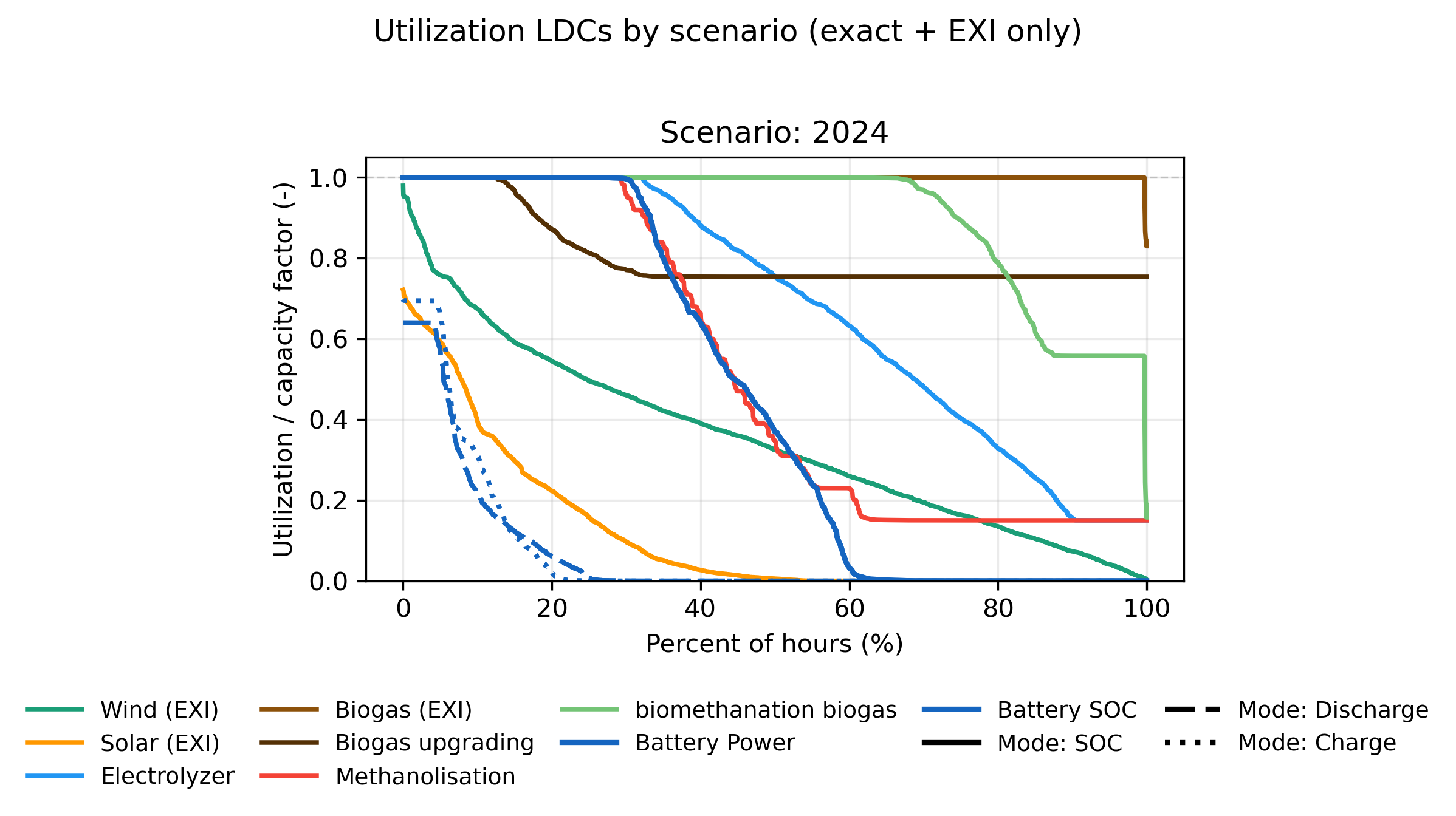
Utilization LDCs under rolling horizon: the same capacity profile as Tutorial 2, now re-dispatched hour-by-hour with a 168 h lookahead window.#
—
4 · PF vs RH — operation patterns side by side#
The aggregate cost gap (€112 k/y) is small, but the individual asset dispatch patterns reveal where the differences lie. The figure below shows, for each key component, a day-of-year × hour heatmap comparing PF (left) against RH (right):
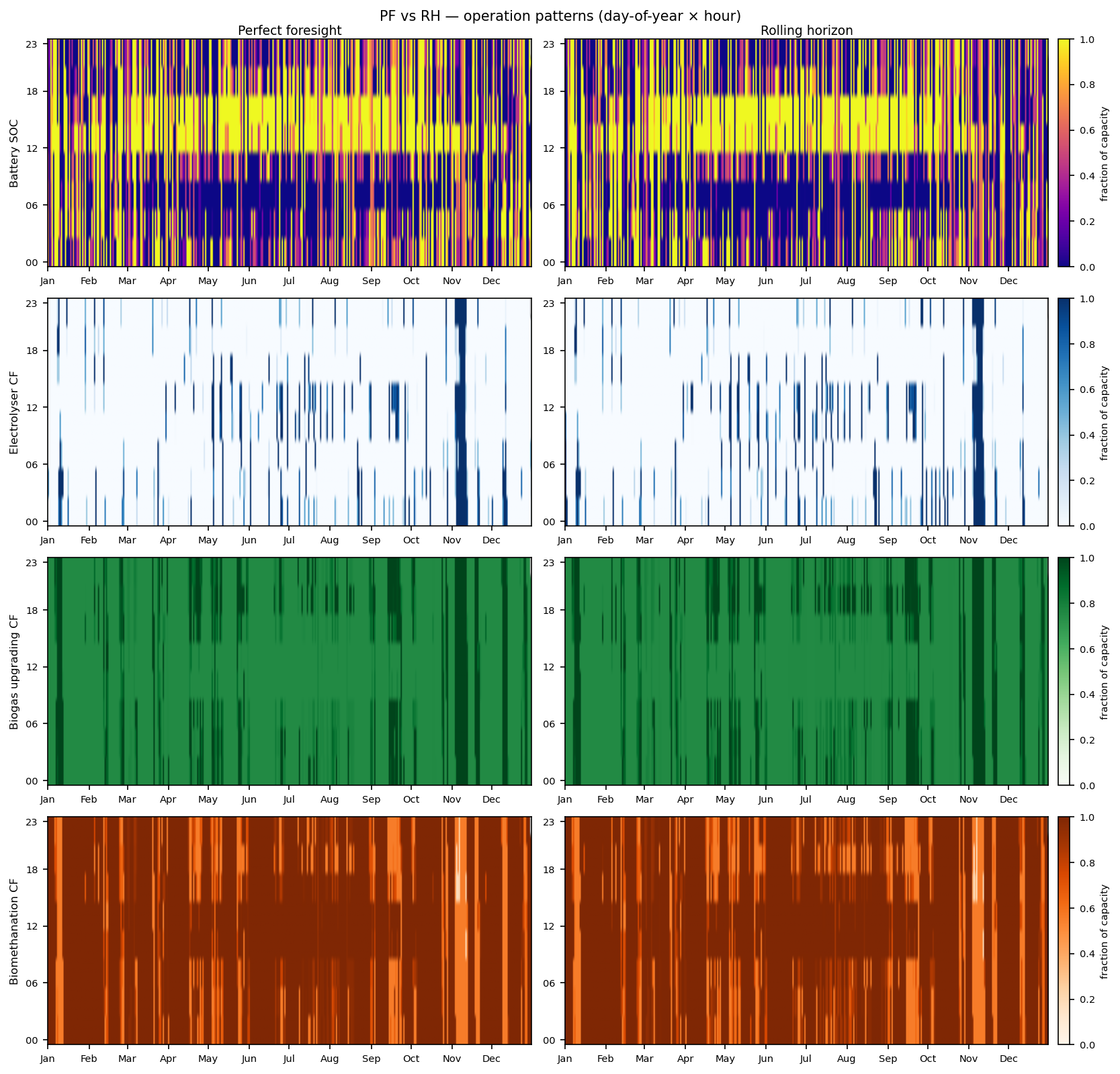
Operation heatmaps — perfect foresight (left) vs rolling horizon (right) for four components. Each cell is the mean capacity factor for that hour-of-day and day-of-year.#
Reading the heatmaps:
Battery SOC — the most visible difference. PF charges the battery with precise timing (notably in summer, when solar surplus is predictable far in advance); RH tends to keep SOC flatter and slightly higher on average because it cannot see more than 168 h ahead and hedges conservatively. Neither pattern is “wrong” — they reflect different information horizons.
Electrolyser CF — both show the same seasonality (more operation in spring/autumn when wind is strong and prices are low), but RH produces a noisier pattern with less clean clustering of cheap-power hours. The small electrolyser (2.5 MW new capacity on top of the brownfield plant) amplifies these timing differences relative to total plant output.
Biogas upgrading CF — nearly identical in PF and RH. Upgrading runs as near-baseload in both cases because its input (biogas from the digester) is continuous and its output has a fixed biomethane demand. No foresight advantage.
Biomethanation CF — also very similar. High-CF baseload operation means the 168 h window is more than enough lookahead; there is nothing to gain from knowing the full year.
The heatmaps confirm the economic conclusion: the battery is the only asset that meaningfully benefits from longer foresight, and with only 2 hours of capacity that benefit is small. Adding a larger thermal or hydrogen store would make the PF–RH gap — and the visual difference in these heatmaps — much larger.
—
What you learned#
The difference between perfect-foresight expansion and rolling-horizon dispatch.
horizon/overlapwindow mechanics and thenetwork_pathinput.Why short-duration storage makes the PF–RH gap small, and when it would widen.
Next: Tutorial 4 — Two-Stage Stochastic Optimisation optimises the investment against several scenarios at once.